Basics#
import numpy as np
import matplotlib.pyplot as plt
import astropy.units as u
from astropy.utils.data import clear_download_cache
clear_download_cache()

from spextra import Spextrum, spextra_database, SpecLibrary, FilterSystem
Examining the database#
sdb = spextra_database
Information of the database#
print(sdb)
Spextra Database:
  Remote URL: https://scopesim.univie.ac.at/spextra/database/
  Local path: /home/docs/.spextra_cache
Database contents:
├─libraries:
│ ├─ref: A library of reference stars
│ ├─kc96: Kinney-Calzetti Atlas
│ ├─pickles: Pickles Stellar Library
│ ├─dobos: SDSS galaxy composite spectra
│ ├─irtf: IRTF spectral library
│ ├─agn: AGN templates
│ ├─nebulae: Emission line nebulae
│ ├─brown: Galaxy SEDs from the UV to the Mid-IR
│ ├─kurucz: Subset of Kurucz 1993 Models
│ ├─sne: Supernova Legacy Survey
│ ├─moehler: flux/telluric standards with X-Shooter
│ ├─madden: High-Resolution Spectra of Habitable Zone Planets
│ ├─bosz/hr: BOSZ stellar atmosphere Grid - High Resolution
│ ├─bosz/mr: BOSZ stellar atmosphere Grid - Medium Resolution
│ ├─bosz/lr: BOSZ stellar atmosphere Grid - Low Resolution
│ ├─assef: Low-resolution spectral templates for AGN and galaxies
│ ├─sky: Paranal sky background spectra
│ ├─shapley: Rest-Frame Ultraviolet Spectra of z ∼ 3 Lyman Break Galaxies
│ ├─etc/kinney: ESO ETC version of the Kinney-Calzetti Atlas
│ ├─etc/kurucz: ESO ETC subset of the Kurucz 1993 models
│ ├─etc/marcs/p: ESO ETC subset of the MARCS Stellar Models with Plane Parallel Geometry
│ ├─etc/marcs/s: ESO ETC subset of the MARCS Stellar Models with Spherical Geometry
│ ├─etc/misc: Other templates, nubulae and qso
│ └─etc/pickles: ESO ETC subset of the Pickles stellar library
├─extinction_curves:
│ ├─gordon: LMC and SMC extinction laws
│ ├─cardelli: MW extinction laws
│ └─calzetti: extragalactic attenuation curves
└─filter_systems:
  ├─elt/micado: MICADO filters
  ├─elt/metis: METIS filters
  └─etc: ESO ETC standard filters
# Which templates are available?

print(SpecLibrary("sne"))
Downloading file 'libraries/sne/index.yml' from 'https://scopesim.univie.ac.at/spextra/database/libraries/sne/index.yml' to '/home/docs/.spextra_cache'.
0%| | 0.00/1.03k [00:00<?, ?B/s]
0%| | 0.00/1.03k [00:00<?, ?B/s]
100%|██████████████████████████████████████| 1.03k/1.03k [00:00<00:00, 869kB/s]
Spectral Library 'sne': Supernova spectral library
  spectral coverage: uv, vis, nir
  wave_unit: Angstrom
  flux_unit: FLAM
  Templates: sn1a, sn1b, sn1c, sn2l, sn2p, sn2n, hyper, pop3_3d, pop3_15d
Extinction curves and Filters#
print(sdb["extinction_curves"])
print(sdb["filter_systems"])
{'gordon': 'LMC and SMC extinction laws', 'cardelli': 'MW extinction laws', 'calzetti': 'extragalactic attenuation curves'}
{'elt/micado': 'MICADO filters', 'elt/metis': 'METIS filters', 'etc': 'ESO ETC standard filters'}
print(FilterSystem("micado"))
Filter system 'micado': <untitled>
  spectral coverage:
  wave_unit: Angstrom
  filters:
Retrieving the spectra#
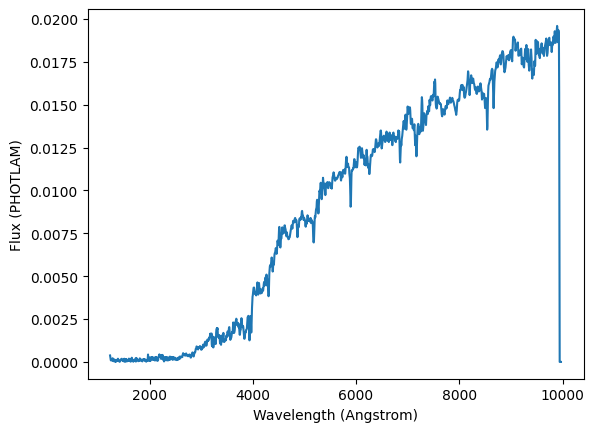
sp1 = Spextrum("kc96/s0")
sp1.plot()
Downloading file 'libraries/kc96/s0.fits' from 'https://scopesim.univie.ac.at/spextra/database/libraries/kc96/s0.fits' to '/home/docs/.spextra_cache'.
0%| | 0.00/20.2k [00:00<?, ?B/s]
36%|█████████████▏ | 7.17k/20.2k [00:00<00:00, 62.3kB/s]
0%| | 0.00/20.2k [00:00<?, ?B/s]
100%|█████████████████████████████████████| 20.2k/20.2k [00:00<00:00, 24.8MB/s]
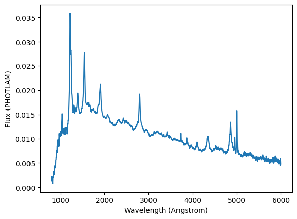
# another spectrum

sp2 = Spextrum("agn/qso")
sp2.plot()
Downloading file 'libraries/agn/index.yml' from 'https://scopesim.univie.ac.at/spextra/database/libraries/agn/index.yml' to '/home/docs/.spextra_cache'.
0%| | 0.00/2.19k [00:00<?, ?B/s]
0%| | 0.00/2.19k [00:00<?, ?B/s]
100%|█████████████████████████████████████| 2.19k/2.19k [00:00<00:00, 1.86MB/s]
Downloading file 'libraries/agn/qso.fits' from 'https://scopesim.univie.ac.at/spextra/database/libraries/agn/qso.fits' to '/home/docs/.spextra_cache'.
0%| | 0.00/23.0k [00:00<?, ?B/s]
62%|███████████████████████▋ | 14.3k/23.0k [00:00<00:00, 125kB/s]
0%| | 0.00/23.0k [00:00<?, ?B/s]
100%|█████████████████████████████████████| 23.0k/23.0k [00:00<00:00, 19.8MB/s]
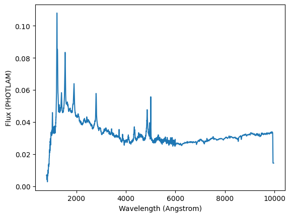
Aritmetics#
simple arithmetics are possible
sp = sp1 + 3*sp2

sp.plot()
Adding emission lines#
It is possible to add emission lines, either individually or as a list. Parameters are center, flux and fwhm
sp3 = sp1.add_emi_lines(center=4000,flux=4e-13, fwhm=5*u.AA)
sp3.plot(left=3500, right=4500)

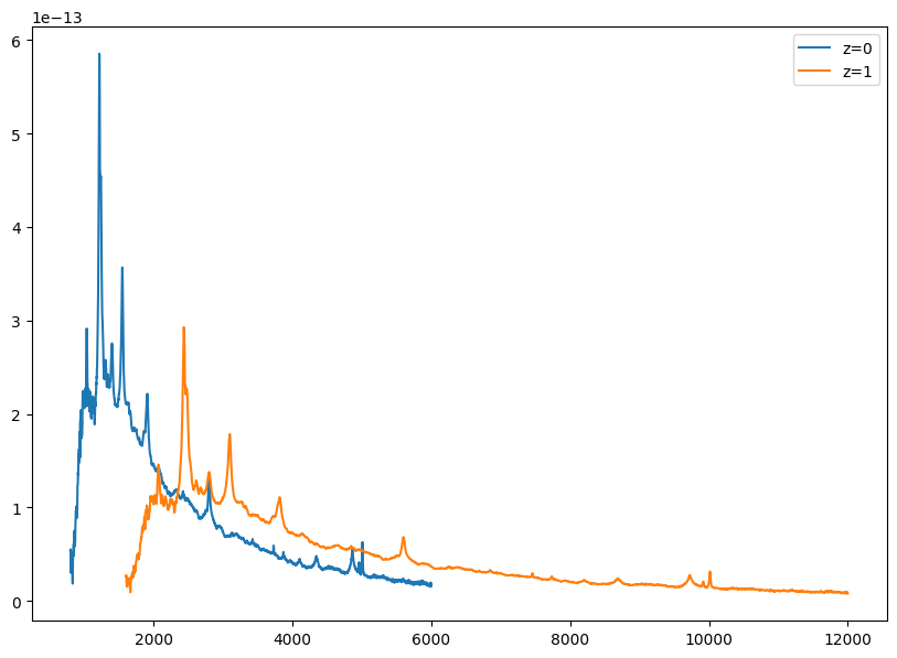
Redshifting spectra#
fig = plt.figure(figsize=(10,7))
sp4 = sp2.redshift(z=1)

wave = sp2.waveset
flux = sp2(wave, flux_unit="FLAM")

plt.plot(wave, flux)

plt.plot(sp4.waveset,
         sp4(sp4.waveset, flux_unit="FLAM"))

plt.legend(['z=0', 'z=1'], loc='upper right')
<matplotlib.legend.Legend at 0x7f66754511d0>
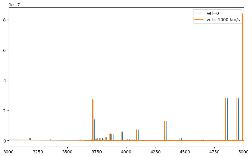
Or using velocity#
fig = plt.figure(figsize=(10,6))

sp1 = Spextrum("nebulae/orion")

vel = -1000 * u.km / u.s
sp2 = sp1.redshift(vel=vel)

plt.plot(sp1.waveset,
         sp1(sp1.waveset, flux_unit="FLAM"))
plt.plot(sp2.waveset,
         sp2(sp2.waveset, flux_unit="FLAM"))
plt.legend(['vel=0', 'vel=-1000 km/s'], loc='upper right')
plt.xlim(3000,5000)
Downloading file 'libraries/nebulae/index.yml' from 'https://scopesim.univie.ac.at/spextra/database/libraries/nebulae/index.yml' to '/home/docs/.spextra_cache'.
0%| | 0.00/1.51k [00:00<?, ?B/s]
0%| | 0.00/1.51k [00:00<?, ?B/s]
100%|█████████████████████████████████████| 1.51k/1.51k [00:00<00:00, 1.28MB/s]
Downloading file 'libraries/nebulae/orion.fits' from 'https://scopesim.univie.ac.at/spextra/database/libraries/nebulae/orion.fits' to '/home/docs/.spextra_cache'.
0%| | 0.00/170k [00:00<?, ?B/s]
4%|█▌ | 7.17k/170k [00:00<00:02, 63.4kB/s]
14%|█████▋ | 24.6k/170k [00:00<00:01, 114kB/s]
25%|█████████▊ | 43.0k/170k [00:00<00:00, 136kB/s]
45%|█████████████████▍ | 75.8k/170k [00:00<00:00, 195kB/s]
64%|█████████████████████████▌ | 109k/170k [00:00<00:00, 227kB/s]
0%| | 0.00/170k [00:00<?, ?B/s]
100%|████████████████████████████████████████| 170k/170k [00:00<00:00, 243MB/s]
(3000.0, 5000.0)
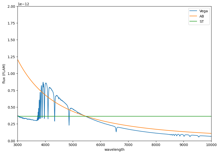
Flat spectrum in any photometric system#
(aka reference spectrum if mag=0)
sp_vega = Spextrum.flat_spectrum(10*u.mag)
sp_ab = Spextrum.flat_spectrum(10*u.ABmag)
sp_st = Spextrum.flat_spectrum(10*u.STmag)


fig = plt.figure(figsize=(10,7))
wave = sp_vega.waveset
plt.plot(wave, sp_vega(wave, flux_unit="FLAM"), label="Vega")
plt.plot(wave, sp_ab(wave, flux_unit="FLAM"), label="AB")
plt.plot(wave, sp_st(wave, flux_unit="FLAM"), label="ST")

plt.xlim(3000,1e4)
plt.ylim(0,0.2e-11)
plt.xlabel("wavelength")
plt.ylabel("flux (FLAM)")
plt.legend()
Downloading file 'libraries/ref/vega.fits' from 'https://scopesim.univie.ac.at/spextra/database/libraries/ref/vega.fits' to '/home/docs/.spextra_cache'.
0%| | 0.00/276k [00:00<?, ?B/s]
5%|██ | 14.3k/276k [00:00<00:02, 126kB/s]
16%|██████ | 43.0k/276k [00:00<00:01, 199kB/s]
27%|██████████▋ | 75.8k/276k [00:00<00:00, 238kB/s]
45%|██████████████████ | 125k/276k [00:00<00:00, 312kB/s]
63%|█████████████████████████▏ | 174k/276k [00:00<00:00, 353kB/s]
81%|████████████████████████████████▎ | 223k/276k [00:00<00:00, 378kB/s]
0%| | 0.00/276k [00:00<?, ?B/s]
100%|████████████████████████████████████████| 276k/276k [00:00<00:00, 423MB/s]
<matplotlib.legend.Legend at 0x7f6675357490>
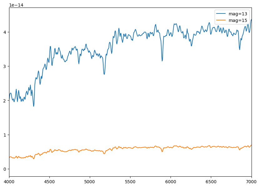
Scaling to a magnitude#
sp1 = Spextrum("kc96/s0").scale_to_magnitude(amplitude=13 * u.ABmag, filter_curve="g")
sp2 = sp1.scale_to_magnitude(amplitude=15 * u.ABmag, filter_curve="g")

sig = plt.figure(figsize=(10,7))
plt.plot(sp1.waveset,
         sp1(sp1.waveset, flux_unit="FLAM"))
plt.plot(sp2.waveset,
         sp2(sp2.waveset, flux_unit="FLAM"))
plt.legend(['mag=13', 'mag=15'], loc='upper right')
plt.xlim(4000,7000)
(4000.0, 7000.0)
Obtaining magnitudes from spectra#
print("Magnitude spectra 1:", sp1.get_magnitude(filter_curve="g"),
      sp1.get_magnitude(filter_curve="g", system_name="Vega"), "Vega")
print("Magnitude spectra 2:", sp2.get_magnitude(filter_curve="g"),
      sp2.get_magnitude(filter_curve="g", system_name="Vega"), "Vega")
Magnitude spectra 1: 13.0 mag(AB) 13.095325163298817 mag Vega
Magnitude spectra 2: 15.0 mag(AB) 15.095325163298817 mag Vega
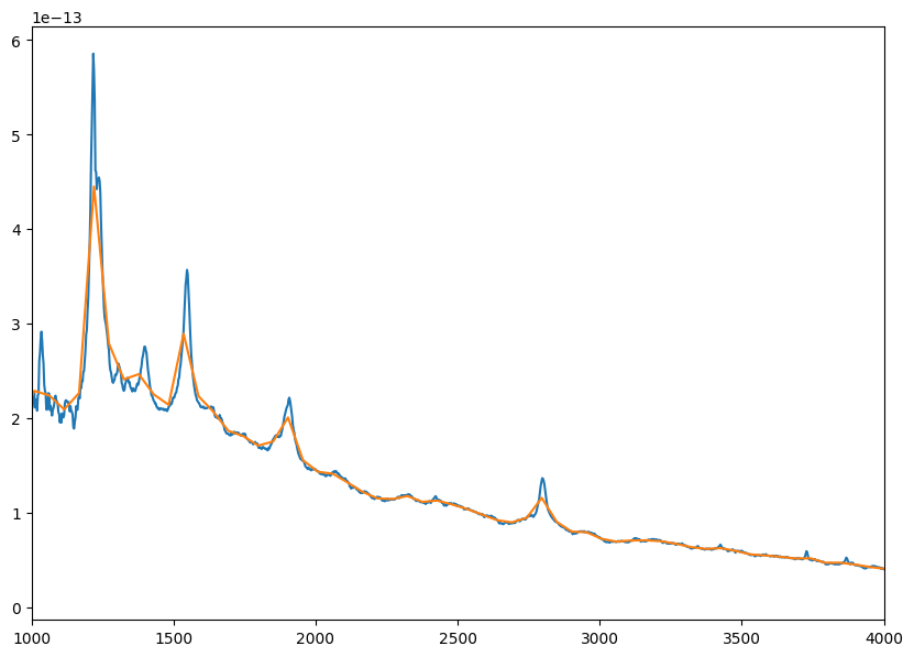
Rebin spectra#
a new wavelength array must be passed
sp1 = Spextrum("agn/qso")
new_waves = np.linspace(np.min(sp1.waveset),
                        np.max(sp1.waveset),
                        100)
sp2 = sp1.rebin_spectra(new_waves=new_waves)

sig = plt.figure(figsize=(10,7))
plt.plot(sp1.waveset,
         sp1(sp1.waveset, flux_unit="FLAM"))
plt.plot(sp2.waveset,
         sp2(sp2.waveset, flux_unit="FLAM"))
plt.xlim(1000,4000)
(1000.0, 4000.0)
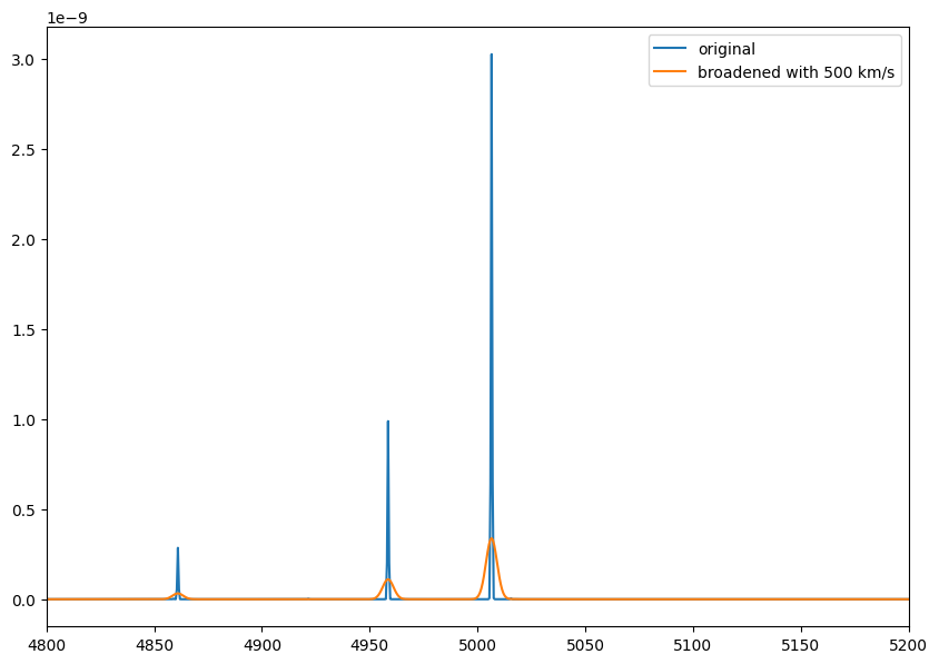
Smooth the spectral with a velocity kernel#
sp1 = Spextrum("nebulae/pn")

sigma = 500*(u.km / u.s)
sp2 = sp1.smooth(sigma=sigma)

fig = plt.figure(figsize=(10,7))
plt.plot(sp1.waveset,
         sp1(sp1.waveset, flux_unit="FLAM"), label="original")
plt.plot(sp2.waveset,
         sp2(sp2.waveset, flux_unit="FLAM"), label="broadened with 500 km/s")

plt.xlim(4800,5200)
plt.legend()
Downloading file 'libraries/nebulae/pn.fits' from 'https://scopesim.univie.ac.at/spextra/database/libraries/nebulae/pn.fits' to '/home/docs/.spextra_cache'.
0%| | 0.00/170k [00:00<?, ?B/s]
4%|█▌ | 7.17k/170k [00:00<00:02, 63.3kB/s]
14%|█████▋ | 24.6k/170k [00:00<00:01, 115kB/s]
27%|██████████▌ | 46.1k/170k [00:00<00:00, 148kB/s]
46%|█████████████████▊ | 77.8k/170k [00:00<00:00, 198kB/s]
59%|███████████████████████▌ | 100k/170k [00:00<00:00, 197kB/s]
88%|███████████████████████████████████▏ | 150k/170k [00:00<00:00, 275kB/s]
0%| | 0.00/170k [00:00<?, ?B/s]
100%|████████████████████████████████████████| 170k/170k [00:00<00:00, 140MB/s]
<matplotlib.legend.Legend at 0x7f6677185f90>
Blackbody spectrum and extinction curves#
sp1 = Spextrum.black_body_spectrum(temperature=5500,
                                   amplitude=10 * u.ABmag,
                                   filter_curve="r")
sp2 = sp1.redden("gordon/smc_bar", Ebv=0.15)


fig = plt.figure(figsize=(10,7))
plt.plot(sp1.waveset,
         sp1(sp1.waveset, flux_unit="FLAM"), label="original")
plt.plot(sp2.waveset,
         sp2(sp2.waveset, flux_unit="FLAM"), label="attenuated")

plt.xlim(1800,15200)
plt.legend()
---------------------------------------------------------------------------
AttributeError                            Traceback (most recent call last)
File ~/checkouts/readthedocs.org/user_builds/spextra/envs/latest/lib/python3.11/site-packages/astropy/units/decorators.py:73, in _validate_arg_value(param_name, func_name, arg, targets, equivalencies, strict_dimensionless)
     72 try:
---> 73     if arg.unit.is_equivalent(allowed_unit, equivalencies=equivalencies):
     74         break

AttributeError: 'int' object has no attribute 'unit'

During handling of the above exception, another exception occurred:

TypeError                                 Traceback (most recent call last)
Cell In[18], line 1
----> 1 sp1 = Spextrum.black_body_spectrum(temperature=5500,
      2                                    amplitude=10 * u.ABmag,
      3                                    filter_curve="r")
      4 sp2 = sp1.redden("gordon/smc_bar", Ebv=0.15)
      7 fig = plt.figure(figsize=(10,7))

File ~/checkouts/readthedocs.org/user_builds/spextra/envs/latest/lib/python3.11/site-packages/astropy/units/decorators.py:302, in QuantityInput.__call__.<locals>.wrapper(*func_args, **func_kwargs)
    294         valid_targets = [
    295             t
    296             for t in valid_targets
    297             if isinstance(t, (str, UnitBase, PhysicalType))
    298         ]
    300     # Now we loop over the allowed units/physical types and validate
    301     #   the value of the argument:
--> 302     _validate_arg_value(
    303         param.name,
    304         wrapped_function.__name__,
    305         arg,
    306         valid_targets,
    307         self.equivalencies,
    308         self.strict_dimensionless,
    309     )
    311 # Call the original function with any equivalencies in force.
    312 with add_enabled_equivalencies(self.equivalencies):

File ~/checkouts/readthedocs.org/user_builds/spextra/envs/latest/lib/python3.11/site-packages/astropy/units/decorators.py:82, in _validate_arg_value(param_name, func_name, arg, targets, equivalencies, strict_dimensionless)
     79         else:
     80             error_msg = "no 'unit' attribute"
---> 82         raise TypeError(
     83             f"Argument '{param_name}' to function '{func_name}'"
     84             f" has {error_msg}. You should pass in an astropy "
     85             "Quantity instead."
     86         )
     88 else:
     89     error_msg = (
     90         f"Argument '{param_name}' to function '{func_name}' must "
     91         "be in units convertible to"
     92     )

TypeError: Argument 'temperature' to function 'black_body_spectrum' has no 'unit' attribute. You should pass in an astropy Quantity instead.
Photons within a filter#
(or between wmin or wmax)
n_photons = sp2.photons_in_range(area=2*u.m**2,
                                 filter_curve="V")

print(n_photons)